How Much Wood Could a Woodchuck Chuck if a Woodchuck Weighed 850 lbs? Why Linear Regressions Fail At Extrapolation

The BLS uses HQA to evaluate a new product using the pricing relationships that existed in the past to value what the new product would have cost in the past. Setting aside the myriad of fundamental arguments one could make against this process, lets look at a bonafide statistical pitfall that Hedonic Quality Regression (HQR) fails to address. At best this introduces a bias into the CPI, and at worst renders the prices used completely misleading.

HQR was introduced by economists to tackle a very real problem: products keep changing configuration with each new cycle. Very few products stay exactly the same throughout time; companies a constantly adding new features as technological boundaries are pushed to new limits.

However, technology has a tendency to create things we have never seen before. We can all find a point where a technology we take for granted today didn’t exist in the past. From the telegraph to the internet to the iPad, these were all completely new products at one point with little to no historical pricing data. This means whenever a product is released that is truly different, BLS economists have to use the HQR to extrapolate what the price of this unique object would have been had it existed in the past. If this sounds like nonsense, it is: statistically and intuitively. 

The statistical model that the BLS uses in its HQR’s is called Ordinary Least Squares (OLS), one of the simplest forms of linear regression and something covered in every econometrics 101 class. OLS is basically the children’s toy of statistical models; it is introduced to neonatal econometricians to get them used to how bigger and better models might work.

As you might expect, OLS has severe limitations, but today we will focus on one: the model’s complete failure to extrapolate. Intuitively this means that OLS works best when its presented with data that looks like data it has seen before. When an OLS model encounters data outside the bounds of its understanding, it yields completely nonsensical results.

Performing extrapolation relies strongly on the regression assumptions. The further the extrapolation goes outside the data, the more room there is for the model to fail due to differences between the assumptions and the sample data or the true values

– proverb

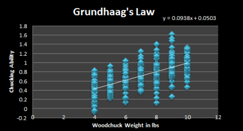
To provide an illustration of this effect, let’s consider a world in which the mythical wood chucking woodchuck is an economic reality: competitive wood chucking is big business drawing millions of viewers. The pioneering work of Dr Olaf Grundhaag established that their is a strong linear statistical relationship between woodchuck weights (which range between 4-10 lbs) and wood chucking ability as measured in board feet of wood. Now know as Grundhaag’s Law, the relationship can be summarized in the now famous graph:

As you might imagine, breeding champion chuckers has become very competitive business. One enterprising breeder retains the services of Korean cloning sensation Dr. Hwang Woo-Suk to splice grizzly bear DNA into a woodchuck embryo, which is gestated via implant by a trained circus bear named Bubbles.

Bubbles gives birth to an enormous woodchuck with unknown wood chucking abilities. It reaches chucking maturity weighing in at 850 lbs. Rather than risk annihilation via wood hurled by his monster woodchuck, the breeder retains the services of Dr. Grundhaag to estimate the wood chucking prowess of the bear-chuck hybrid. This information will be used to build a custom training enclosure.

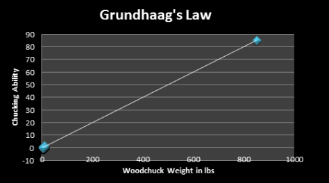
Knowing the limitations of OLS regression, Dr. Grundhaag faces a classic principal-agent problem: he knows that the predictive power of his model is suspect given the weight of the bear-chuck is so far out of the previous weight range for woodchucks (4-10 lbs). However, he doesn’t want to let easy money slip through his fingers or, worse yet, look stupid when he says his model can’t handle the task. So he steps up to the plate and plugs 850 lbs into his model:

Dr Grundhaag cautiously delivers his prediction to the breeder: 85 board feet of chucking ability (a decent sized tree)! The breeder is so excited he orders 5 more monster bearchucks. However, the breeder is shocked when the bearchuck tears his arm clear out of the socket trying to chuck a champion tree. What the hell went wrong? The breeder is ruined. Contemplating a mixture of revenge and suicide, the breeder phones Dr. Grundhaag at a conference and asks “Why did your prediction fail?”

Grundhaag’s model failed because of something called non-linearity. When woodchucks weigh between 4-10 lbs, the relationship between ability and weight looks linear. Adding 1 lb to your chuck always creates the same change in chucking ability. But adding over 800 lbs to your chuck is bound to create some instabilities.

This is a fact of nature — scale matters. If you invented an anti-shrink ray gun and scaled up an ant up to the size of a football stadium, it wouldn’t be able to lift 10 times its body weight… it might not even be able to lift itself. The structure of an ants body was made for its size. Look at the health problems faced by gigantic humans.

Its the same with giant bearchuck hybrids; they just can’t take the strain of slinging a redwood, as predicted by Grundhaag’s Law. Sure, they can chuck more wood than any woodchuck in the history of chucking, just not as much as a linear relationship would suggest extrapolated from a completely different range of input data.

Coming back to reality, when a manufacturer discontinues a product or introduces a completely new product to the marketplace, the BLS is doing the equivalent of applying Grundhaag’s Law.  They extrapolating outside the range of data previously used to create the Hedonic Quality Regressions. The results are to be taken with big, fat granules of salt. In other words, the results cannot be trusted. Nor can they be verified, since the BLS keeps data such as this under lock and key.

CPI Market Basket Determined by only 0.006% of Americans

It seems like every week we discover a new way in which our daily lives are being tracked. Every phone-call, text, e-mail, credit card transaction, even every web-page we ever visit can be intercepted and archived. That’s why it seems like a quaint throwback that the CPI market basket is computed from a self-reported survey of 0.006% of American Households.

The market basket is determined from the Consumer Expenditure (CE) Survey, conducted on the BLS’s behalf by the Census Bureau. This information is supplemented by the Telephone Point of Purchase (TPOP) Survey, an old-fashion telephone survey conducted by the Census. 

Considering the massive liabilities that are tied to the computation of the CPI, using antiquated methods of data collection seems at best reckless, at worst criminally negligent. There are several reasons that the current method is dubious.

Using statistical sampling introduces an amount of error in the quantity you are trying to measure. The logic is that sampling all 316 million US citizens would be prohibitively expensive so pick a smaller sample that is still representative of the overall population. The BLS has chosen a very small sample of 7000 households, making it imperative that their assumptions are correct. Given the monotonicity of thought amongst BLS economists, it would not be surprising if what they thought was representative was in fact biased.

A combination of academic arrogance combined with constrained budgets leads me to question how representative the market basket is of the wider population it is meant to measure. This need not be the case, as spending data is available for purchase from major credit card providers. Taking a census is expensive and inefficient. Additionally, there doesn’t seem to be any thought given to the measurement error inherent in self-reported and phone surveys.

It is unlikely that people record their true purchases; reporting instead an idealized image of what they think they should have purchased. No one is going to accurately report the amount of alcohol, cigarettes, cheese-burgers, candy, soft-drinks, green tea, kale, exercise, travel or whatever else they use to numb the reality of everyday existence. For an everyday example of this phenomenon, look at anyone’s facebook page. Human beings project their own self-image into the data they report to the world (and even themselves), and the CE survey is no different.

Using anonymous spending data filtered from credit card processors would solve several problems at once:

• It would provide researchers access to a much larger sample of the population and make the CPI market basket much a more accurate representation of individual spending habits.
• It would eliminate much of the measurement error associated with current survey methods. Your credit card statement is much more objective than a phone survey.

Publicly available pricing information should also be included, and would provide a more nuanced and accurate picture of how inflation is evolving in the broader economy.

Sources:
http://quickfacts.census.gov/qfd/states/00000.html
http://www.bls.gov/cpi/cpifaq.htm#Question_6
http://www.bls.gov/respondents/cpi/tpops/home.htm

Use of Hedonic Quality Adjustments: Country by Country

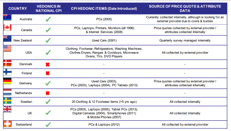
This table neatly summarizes the use of Hedonic Quality Regressions worldwide:

Source: http://www.ons.gov.uk/ NB: The USA also uses quality adjustments in owner equivalent rent calculations (representing ~ 25% of all-items CPI)

Quality Adjusted CPI Saved the Federal Government at least $150 Billion from 1998-2012

Cost-of-living adjustments increase entitlement spending automatically every year. Most COLA’s use all or part of the CPI to calculate inflation. The US further embeds the CPI in the system by indexing a growing portion of its government debt via TIPs. Even welfare benefits like food stamps use applicable indices within the all-items CPI to calculate COLA.

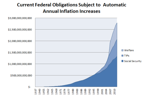
In total almost $3 trillion of federal yearly liability is subject to automatic annual CPI-based increases. This calculation includes:

• All yearly means-tested welfare benefits subject to a COLA (e.g. SNAP, NSLP, etc…)
• All yearly social security spending (e.g. SSI, OASI, DI, everything…)
• All outstanding TIPs balance (every year the principal of an outstanding TIP is adjusted up/down by the inflation rate)

sources: http://budget.house.gov/uploadedfiles/rectortestimony04172012.pdf
http://www.ssa.gov/policy/docs/statcomps/supplement/index.html
http://www.gpo.gov/fdsys/pkg/ERP-2012/xls/ERP-2012-table87.xls

This time series represents the majority of yearly federal obligations that are subject to inflation-based COLA increases. We can thus attempt to calculate how much the government saved each year through methodological changes to the CPI. By the government’s own reckoning:

[The] improvements made by the BLS have reduced the measured
increase in the CPI… The combined effect of the changes made through 1998 has been to lower the CPI inflation rate by 0.44 percentage point per year. Changes to be implemented in 1999 and 2000 will lower CPI inflation by a further 0.20 and 0.04 percentage point per year.

– Economic Report of the President Feb 1999 pg 93

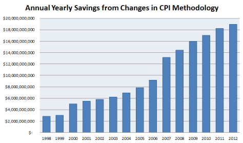
Thats a total of 0.68% a year from 2000 onward. While this might not sound like a lot, given the immense sums of money the government owes the public, this adds up to billions of dollars in savings:

applies deflation rate implied from report (0.0044 in 1998 up to 0.0068 in 2000) to total obligations calculated above

That adds up to a total savings of $150,147,988,800. Again, this is basing our deflation rate at 0.68% from the economic report referenced above. There is considerable evidence, however, that the real effect of quality adjustments on the CPI is much higher.

Using the more realistic divergence of 1-2% we saw from the BPP data puts the total savings at the $200-$400 billion range. 

In the investigation of any crime, it is important to find motive:

• When a seemingly trivial change to a statistical index can potentially deprive taxpayers of hundreds of billions of dollars 
• When an agency keeps raw data hidden from outside inspection (BLS deems raw pricing data as confidential and thus exempt from FOIA)
• When a government cannot make the unpopular decisions necessary to reign in entitlement spending

Then you are in a time where an executive branch might take actions into its own hands in the name of efficiency. Hiding in econometric obscurity, in an area of research so boring no economist would dare tread, did the government knowingly encourage the adoption of a dubious economic theory that would likely bias inflation downward? If so, it was a good bet.

Estimating the Effect of Hedonic Quality Adjustments on the Consumer Price Index

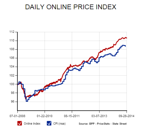
Having an informed debate over Hedonic Quality Adjustments is difficult due to the lack of comparable consumer price indices. A few exist, however, and today we will look at an index compiled by PriceStats, an off-shoot of MIT’s Billion Prices Project, which scrapes the internet for prices and compiles a daily index that aims to track inflation in real-time.

The time series eschews hedonic and seasonal adjustments and relies on sampling over 5 million products to produce a very different look at inflation (CPI included for comparison):

Since starting calculation of the index in mid-2008, PriceStats inflation series has remained consistently above the CPI as reported by the BLS. Considering the differences in methodology this provides an estimate to how much Hedonic Quality Adjustments have been used to understate the head-line CPI figures. Currently, the CPI uses quality adjustments on over 32% of the items used in its calculation. 

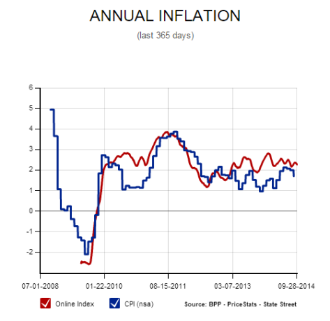
Annual inflation figures show a similar story, occasionally showing divergences greater than 1.5% in the two measures of annual inflation:

In addition to being used as a benchmark for policymaker’s worldwide, CPI’s influence a myriad of payments:

• calculating cost-of-living adjustments to social security and federal retirement programs,
• calculating payments on over $700 billion worth of inflation protected securities (TIPs)
• determining pay-bands in public and private entities
• cost of living adjustments to collective bargaining agreements
• determining IRS tax brackets and numerous tax-related levels (exemptions, for example)
• Basic CPI indices feed into the PCE price index which is the preferred measure of inflation by the FOMC

Overall, CPI’s are used to index payments on over $10 trillion in liabilities. Any underestimation of  CPI benefits the federal government at the expense of the taxpayer and amounts to a backdoor default on its financial obligations. Please understand this could be deliberate or the result of dubious econometric methods. Using a bad model is like using a random number generator as a compass. 

To get an idea of the sums of money involved, for every 1% of CPI underestimation the federal government saves $8.4 billion on social security payments alone.  The lack of transparency regarding quality adjustments (and their perceived complexity) provides a perfect smoke-screen for covert debt management through CPI under-reporting.

There is no reason for this to be the case. Hedonic Quality Adjustments are computed via linear regressions, one of the least complicated models in statistics. Any statistician provided with the data could verify the BLS’s regressions using an off-the-shelf statistical computing package like R. Release the data, plain and simple; any other response smacks of corruption in the name of regression or an attempt to justify one’s existence.

32% of the Products Used in BLS Consumer Price Index Subject to Hedonic Quality Adjustments

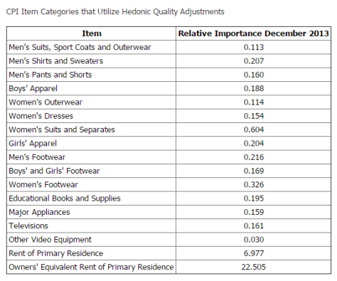
A full 32.48% of the items included in the CPI are subject to Hedonic Quality Adjustments; 3% from consumer products and over 29% from housing. With inflation targets in the 2% range, even a small error in estimating Hedonic Quality Regressions could severely bias policymakers’ perceptions of reality. 

Source: http://www.bls.gov/cpi/cpihqaitem.htm

Manipulating the Consumer Price Index: Hedonic Quality Adjustments

Have you heard the one about CPI?

Suppose that a TV manufacturer retires a product and replaces it with a newer, better, and much more expensive one. If the new TV costs 5 times more than the old one, how can we gently massage the price of the old TV to make it look like the price fell? By using the dark arts of econometrics, my son!

If you believe the public comments made by the world’s central bankers, the prices that consumers pay for items are not rising fast enough; in some places like Europe they worry that prices might actually fall (a tragedy for the possessing classes, as their manic one-way long bets might not work then). Central bankers are terrified of this outcome. Setting aside for a second the apparent insanity of this logic for your average consumer, who experiences price rises on a near continuous basis, let’s examine in detail one of the gauges economists use for measuring prices: the Consumer Price Index (CPI).

Ostensibly, the CPI is a linear combination of the “prices” of things/stuff consumers could actually purchase weighted by a percentage that the “ideal consumer” spends on any particular stuff/thing in his “ideal” basket. The main problem here is that the “prices” used are not the prices a consumer would actually pay; instead the real price for an item is scaled by what the BLS calls a “Hedonic Quality Adjustment (HQA)”. The HQA was designed to solve a real world problem economists face: the market keeps pumping out new and better devices. In practice the HQA is used to artificially depress the prices used in the calculation of the CPI.

Intuitively, the HQA scales prices by their “perceived” quality. We’re not talking about human perception here, but that of a kitchen sink regression model created by BLS economists. Essentially it throws every quality an item might possess into a linear model and performs a regression of these qualities against the prices found in the market for a given product. The prices that feed into the CPI can be intuitively modeled as:

This means that as far as the CPI is concerned, prices can “decrease” for three reasons:

• The price actually decreases, holding quality constant
• The “quality” as measured by the Hedonic Quality Regression (HQR) could go up, holding price constant
• The “quality” goes up by more than prices go up (<<<<<< WE’RE HERE RIGHT NOW)

In a time of rapid technological development, the quality as measured by HQR will increase by orders of magnitude more than prices. Consider Moore’s Law, which correctly postulated that the number of transistors on computer chips would double every two years; prices can’t possibly keep up with that kind of quality increase (save for hyperinflation, more on that later).

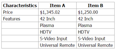
The BLS neatly illustrates this effect with an example from their website (emphasis is mine):

Item A is a television that is no longer available and it has been replaced by a new television, Item B. The characteristics in bold differ between the two TVs. There is a large degree of quality change and there is a very large (400%) difference in the prices of these TVs. Rather than use the 400 percent increase in price between Item A and Item B, the quality adjusted rate of price change is measuredby the ratio of the price of Item B in the current period ($1,250.00) over an estimated price of Item B in the previous period – Item B’.

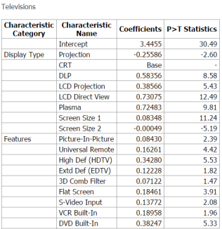
Here is an example of a hedonic regression model (including coefficients) for televisions.

This is just an OLS linear regression model. The dependent variable is the natural log of prices for televisions, the explanatory variables and their coefficients are listed in the table below (most are dummy variables)

Where PB,t+s-1 is the quality adjusted price, PA,t+s-1 is the price of Item A in the previous period, and is the constant e [SIC], the inverse of the natural logarithm, exponentiated by the difference of the summations of the ßs for the set of characteristics that differ between items A and B. The exponentiation step is done to transform the coefficients from the semi log form to a linear form before adjusting the price.

To put it another way, the HQR extrapolates a price for the new TV using the Hedonic Quality model estimated from the population of old TV’s

To derive the estimated price of Item B’, we use the following equation:

For our television example, [the equation above] looks like this:

When this quality adjustment is applied, the ratio of price change looks like this:

The resulting price change is -7.1 percent after the quality adjustment is applied.

Oh good! You see, my neighbor, John Q., thought that prices were going up and was about to riot in the streets because he couldn’t buy anything now. How relieved he was to live next to an economist and mathematician; I merely explained that even though he couldn’t afford the new TV (or anything else) it was actually less expensive once quality was taken into account. Boy was his face red. He went home and explained it to his wife and kids and they laughed and laughed about their mistake.

Few modern people would consider progress to be a bad thing. Quality improvements should be celebrated and technological change embraced. Yet when a policymaker says that she wants inflation to pick up and trots out the CPI as evidence, she doesn’t care whether that comes about from actual price inflation or quality decreases. Given the accelerating pace of technological improvements, it’s hard to imagine an outcome besides hyperinflation that will satisfy central bankers and their slavish dependence on indicators which have been so far abstracted from reality as to have little actionable value.

Alternatively, causing a complete economic meltdown by manipulating the price of money and inflating the mother of all bubbles will probably slow down technological development, so either way, well played.

Since economists are largely concerned with “real” prices (actual prices scaled by inflation as measured by the CPI), any error in the calculation of real prices introduces a bias that propagates to every corner of economic thought. This is a central flaw in economics that largely explains the gap between actual human experiences (“Wow! Things are expensive!”) with central bankers gambling our collective future on fighting deflation.

More than likely the deflation is used as cover for the agency problem faced by central bankers every day. Most market practitioners know we are in a classic debt-fueled bubble initiated by wildly loose monetary policy – central bankers included. Given that the public will rightfully blame policymakers when the bubble bursts, no central banker wants to run the risk that it pops on their watch. That would make them look stupid, and might endanger their future lives as highly paid consultants. In that context printing endless supplies of money makes perfect sense.